Tutorial 1: Unconfined, Semiflexible Homopolymer

This demonstration walks through a simulation of an unconfined, semiflexible homopolymer. In this notebook, we specify a binder, polymer, and field, then we run a simulation. In addition to the setup and evaluation of the simulation, this notebook includes an analysis of end-to-end distance to verify the validity of the model.

Import Modules

Below, we import the built-in, third-party, and custom modules that we need to simulate a semiflexible homopolymer. All simulations require three types of components: binders, polymers, and fields. In this case, we are simulating a homopolymer without binding components. Therefore, we can use the NullBinder class from the binders module as a placeholder. The polymer is an instance of the SSWLC class from the polymers module. Generally speaking, interactions between monomers are handled by the field containing the polymer. In this case, we use the NullField class as a placeholder since we do not have any interacting components. The chromo.mc init file contains the code necessary to run the simulation. The mc_controller module manages the move and selection amplitudes, and the get_unique_subfolder_name function helps us create a unique directory for the simulation results.

# Built-in modules
import os
import sys

# Third-party modules
import numpy as np
import pandas as pd
import matplotlib.pyplot as plt

# Custom modules
from chromo.binders import get_by_name, make_binder_collection
from chromo.polymers import SSWLC
from chromo.fields import NullField
import chromo.mc as mc
import chromo.mc.mc_controller as ctrl
from chromo.util.reproducibility import get_unique_subfolder_name

Specify Binders

Since we do not have any binding components, we will use the NullBinder class as a placeholder. We will instantiate the binder using the get_by_name method from the binders module. The get_by_name method requires the name of the binder as a string. In this case, we specify “null_reader” as the name of the binder.

The make_binder_collection method will produce a Pandas data frame summarizing the binder’s properties, which we refer to as a “binder collection.” A binder collection is necessary to run a simulation.

# Initialize a null binder to serve as a placeholder
null_binder = get_by_name("null_reader")

# Create a binder collection (required to run a simulation)
binder_collection = make_binder_collection([null_binder])

Instantiate the Polymer

Specify the name, number of beads, bead spacing, and persistence length of the polymer. Using these properties, we will initialize a polymer using a Gaussian random walk using the gaussian_walk_polymer class method. The persistence length must be specified as a named argument.

# Specify the name, number of beads, bead spacing, and persistence length of the polymer
name = "poly"
num_beads = 1000
bead_spacings = np.ones(num_beads - 1)
lp = 10

# Instantiate the polymer
poly = SSWLC.gaussian_walk_polymer(name, num_beads, bead_spacings, lp=lp)

No states defined.
No chemical modifications defined.

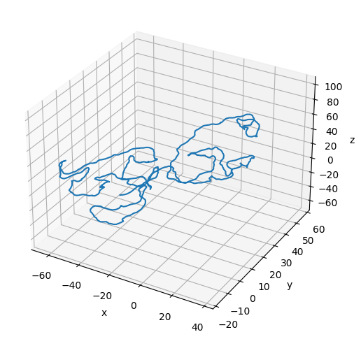
# Plot the initial configuration of the polymer
x = poly.r[:, 0]
y = poly.r[:, 1]
z = poly.r[:, 2]

fig = plt.figure(figsize=(8, 6))
ax = fig.add_subplot(projection='3d')
ax.plot3D(np.asarray(x), np.asarray(y), np.asarray(z))
ax.set_xlabel('x')
ax.set_ylabel('y')
ax.set_zlabel('z')
plt.show()

Instantiate the Null Field

We use the NullField class as a placeholder for the field containing the polymer since we do not have any interacting components.

# The field contains the polymer
field = NullField(polymers=[poly])

Specify the Simulation Parameters

We start by specifying the move and selection amplitudes for the simulation. The move amplitude indicates how large of a transformation each MC move can propose. Specific details about what the move amplitude represents depend on the exact MC move involved. The selection amplitude indicates the maximum number of beads that can be affected by an MC move. How the selection is made depends on the specific moves involved. We can automatically set appropriate amplitudes using the get_amplitude_bounds method of the mc module.

amp_bead_bounds, amp_move_bounds = mc.get_amplitude_bounds(
    polymers = [poly]
)

Since we do not have any binders, we want to evaluate MC moves that only involve geometric transformations. We can do this with the all_moves_except_binding_state methods from the move controller modules. The move selection requires us to specify an output directory to which attempted moves can be logged. We will use the get_unique_subfolder_name function to help us create a new directory for the simulation results. The SimpleController class from the mc_controller module will manage the move and selection amplitudes so that we target 50% acceptance rates for all moves.

out_dir = "output_demo"
latest_sim = get_unique_subfolder_name(f"{out_dir}/sim_")
moves_to_use = ctrl.all_moves_except_binding_state(
    log_dir=latest_sim,
    bead_amp_bounds=amp_bead_bounds.bounds,
    move_amp_bounds=amp_move_bounds.bounds,
    controller=ctrl.SimpleControl
)

To run a simulation, you must specify the number of snapshots and the number of MC steps to attempt per snapshot. The simulation will output the polymer’s configuration at each snapshot.

# Specify the number of snapshots and the number of MC steps to attempt per snapshot
num_snapshots = 200
mc_steps_per_snapshot = 1000

Run the Simulation

Run the simulation by specifying the components of the simulation as well as the simulation parameters. The polymer_in_field method from the mc module will run the simulation. The cell below prints a notification at each save point (these updates have been cleared for this documentation).

polymers = mc.polymer_in_field(
    polymers = [poly],
    binders = binder_collection,
    field = field,
    num_save_mc = mc_steps_per_snapshot,
    num_saves = num_snapshots,
    bead_amp_bounds = amp_bead_bounds,
    move_amp_bounds = amp_move_bounds,
    output_dir = out_dir,
    mc_move_controllers = moves_to_use
)

Analyze the Simulation

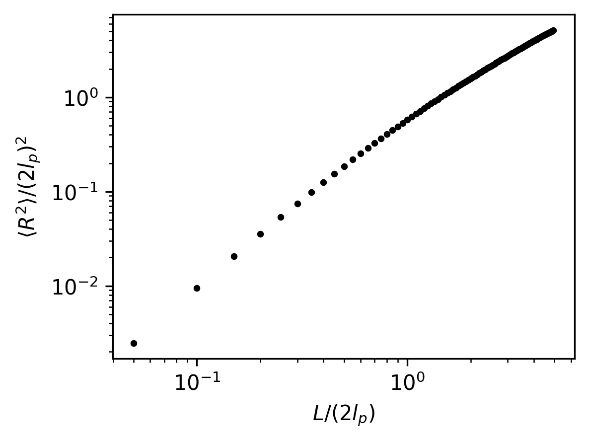
Monte Carlo simulations require a few steps to equilibrate. We will ignore those steps of the MC simulation. Following equilibration, we will analyze the end-to-end distance of the polymer to verify the validity of the model.

# Load the simulation results
sim_dir = latest_sim

# Load and sort snapshots
snapshots = os.listdir(sim_dir)
snapshots = np.array(
    [snap for snap in snapshots if snap.startswith("poly") and snap.endswith(".csv")]
)
snap_inds = np.array([int(snap.split("-")[-1].split(".")[0]) for snap in snapshots])
snapshots = snapshots[np.argsort(snap_inds)]
snap_inds = np.sort(snap_inds)

# Isolate equilibrated snapshots
num_equilibration_steps = 180
snapshots = snapshots[num_equilibration_steps:]

# Specify the segment lengths for which to calculate the end-to-end distances
bead_steps = np.arange(1, 100)
kuhn_steps = bead_steps / (2 * lp)

# Calculate the end-to-end distances for variable segment lengths along the polymer
mean_r2 = []
for i, snap in enumerate(snapshots):
    snap_path = os.path.join(sim_dir, snap)
    config = pd.read_csv(snap_path, sep=",", header=[0, 1], index_col=0)
    r = config["r"].to_numpy()
    mean_r2_snap = []
    for step in bead_steps:
        r1 = r[:-step]
        r2 = r[step:]
        delta_r = r2 - r1
        mean_end_to_end = np.average(np.linalg.norm(delta_r, axis=1) ** 2)
        mean_r2_snap.append(mean_end_to_end)
    mean_r2_snap = np.array(mean_r2_snap)
    mean_r2.append(mean_r2_snap)
mean_r2 = np.array(mean_r2)
mean_r2 = np.average(mean_r2, axis=0)

# Plot the non-dimensionalized mean-squared end-to-end distances
plt.figure(figsize=(4, 3), dpi=300)
plt.scatter(kuhn_steps, mean_r2/((2 * lp)**2), color="black", s=5)
plt.xlabel(r"$L/(2l_p)$")
plt.ylabel(r"$\langle R^2 \rangle / (2l_p)^2$")
plt.xscale("log")
plt.yscale("log")
plt.show()

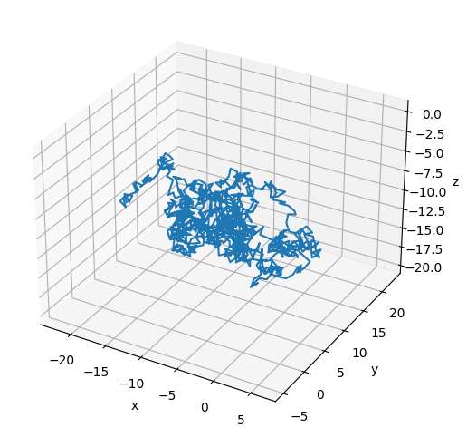
# Plot the final configuration of the polymer
x = polymers[0].r[:, 0]
y = polymers[0].r[:, 1]
z = polymers[0].r[:, 2]

fig = plt.figure(figsize=(8, 6))
ax = fig.add_subplot(projection='3d')
ax.plot3D(np.asarray(x), np.asarray(y), np.asarray(z))
ax.set_xlabel('x')
ax.set_ylabel('y')
ax.set_zlabel('z')
plt.show()