Tutorial 2: Confined, Semiflexible Homopolymer
This tutorial follows from tutorial_1 and will introduce the concept of confinement to the polymer model. The confinement is implemented as a hard spherical boundary. Descriptions of the model setup are included in tutorial_1. This notebook will highlight the addition required to implement the confinement.
Import Modules
[1]:
# Built-in modules
import os
import sys

# Third-party modules
import numpy as np
import pandas as pd
import matplotlib.pyplot as plt

# Custom modules
from chromo.binders import get_by_name, make_binder_collection
from chromo.polymers import SSWLC
from chromo.fields import NullField
import chromo.mc as mc
import chromo.mc.mc_controller as ctrl
from chromo.util.reproducibility import get_unique_subfolder_name
Specify Binders
[2]:
# Initialize a null binder to serve as a placeholder
null_binder = get_by_name("null_reader")

# Create a binder collection (required to run a simulation)
binder_collection = make_binder_collection([null_binder])
Specify the Confinement
We will specify a 2-nm radus spherical confinement. This is a highly confined system, in the context of our polymer.
[3]:
confine_type = "Spherical"
confine_length = 2.0
Instantiate the Polymer
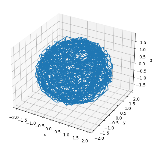
Since we are working in a confined system, we will instantiate the polymer as a random walk inside the confinement using the confined_gaussian_walk class method.
[4]:
# Specify the name, number of beads, bead spacing, and persistence length of the polymer
name = "poly"
num_beads = 1000
bead_spacings = np.ones(num_beads - 1)
lp = 10

# Instantiate the polymer
poly = SSWLC.confined_gaussian_walk(
    name, num_beads, bead_spacings, lp=lp, confine_type=confine_type, confine_length=confine_length
)
No states defined.
No chemical modifications defined.
[5]:
# Plot the initial configuration of the polymer
x = poly.r[:, 0]
y = poly.r[:, 1]
z = poly.r[:, 2]

fig = plt.figure(figsize=(8, 6))
ax = fig.add_subplot(projection='3d')
ax.plot3D(np.asarray(x), np.asarray(y), np.asarray(z))
ax.set_xlabel('x')
ax.set_ylabel('y')
ax.set_zlabel('z')
plt.show()
Instantiate the Null Field
The field is responsible for enforcing the confinement. We need to specify the confinement when we instantiate the field.
[6]:
field = NullField(
    polymers=[poly], confine_type=confine_type, confine_length=confine_length
)
Specify the Simulation Parameters
[7]:
amp_bead_bounds, amp_move_bounds = mc.get_amplitude_bounds(
    polymers = [poly]
)
[8]:
out_dir = "output_demo"
latest_sim = get_unique_subfolder_name(f"{out_dir}/sim_")
moves_to_use = ctrl.all_moves_except_binding_state(
    log_dir=latest_sim,
    bead_amp_bounds=amp_bead_bounds.bounds,
    move_amp_bounds=amp_move_bounds.bounds,
    controller=ctrl.SimpleControl
)
[9]:
# Specify the number of snapshots and the number of MC steps to attempt per snapshot
num_snapshots = 200
mc_steps_per_snapshot = 1000
Run the Simulation
[ ]:
polymers = mc.polymer_in_field(
    polymers = [poly],
    binders = binder_collection,
    field = field,
    num_save_mc = mc_steps_per_snapshot,
    num_saves = num_snapshots,
    bead_amp_bounds = amp_bead_bounds,
    move_amp_bounds = amp_move_bounds,
    output_dir = out_dir,
    mc_move_controllers = moves_to_use
)
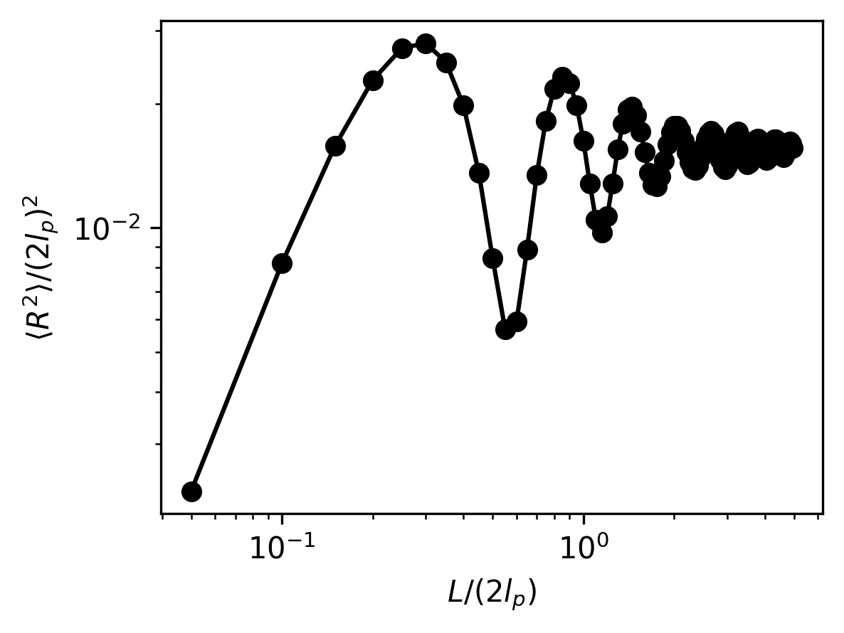
Analyze the Simulation
Again, we will analyze the simulation results by plotting the mean-squared end-to-end distances of the polymer. Notice, oscillations in the mean-squared end-to-end distance emerge as a result of the tight confinement.
[11]:
# Load the simulation results
sim_dir = latest_sim

# Load and sort snapshots
snapshots = os.listdir(sim_dir)
snapshots = np.array([snap for snap in snapshots if snap.startswith("poly") and snap.endswith(".csv")])
snap_inds = np.array([int(snap.split("-")[-1].split(".")[0]) for snap in snapshots])
snapshots = snapshots[np.argsort(snap_inds)]
snap_inds = np.sort(snap_inds)

# Isolate equilibrated snapshots
num_equilibration_steps = 180
snapshots = snapshots[num_equilibration_steps:]
[12]:
# Specify the segment lengths for which to calculate the end-to-end distances
bead_steps = np.arange(1, 100)
kuhn_steps = bead_steps / (2 * lp)

# Calculate the end-to-end distances for variable segment lengths along the polymer
mean_r2 = []
for i, snap in enumerate(snapshots):
    snap_path = os.path.join(sim_dir, snap)
    config = pd.read_csv(snap_path, sep=",", header=[0, 1], index_col=0)
    r = config["r"].to_numpy()
    mean_r2_snap = []
    for step in bead_steps:
        r1 = r[:-step]
        r2 = r[step:]
        delta_r = r2 - r1
        mean_end_to_end = np.average(np.linalg.norm(delta_r, axis=1) ** 2)
        mean_r2_snap.append(mean_end_to_end)
    mean_r2_snap = np.array(mean_r2_snap)
    mean_r2.append(mean_r2_snap)
mean_r2 = np.array(mean_r2)
mean_r2 = np.average(mean_r2, axis=0)
[13]:
# Plot the non-dimensionalized mean-squared end-to-end distances
plt.figure(figsize=(4, 3), dpi=300)
plt.plot(kuhn_steps, mean_r2/((2 * lp)**2), "-o", color="black")
plt.xlabel(r"$L/(2l_p)$")
plt.ylabel(r"$\langle R^2 \rangle / (2l_p)^2$")
plt.xscale("log")
plt.yscale("log")
plt.show()
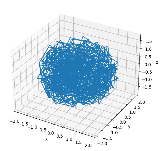
[14]:
# Plot the final configuration of the polymer
x = polymers[0].r[:, 0]
y = polymers[0].r[:, 1]
z = polymers[0].r[:, 2]

fig = plt.figure(figsize=(8, 6))
ax = fig.add_subplot(projection='3d')
ax.plot3D(np.asarray(x), np.asarray(y), np.asarray(z))
ax.set_xlabel('x')
ax.set_ylabel('y')
ax.set_zlabel('z')
plt.show()